Bonds and Spectra: Exercise 3 (Python)

[LuukUnger]

Hi,

In exercise 3 we’re asked to simulate a 1D chain of size N.
I’m having the issue that my histograms differ from those in the answer sheet. It seems to be that the histograms from the answer sheet are cut off version from mine. I’ve looked at it for quite a while now and tried different things but can’t seem to replicate your answers.

My derivation:

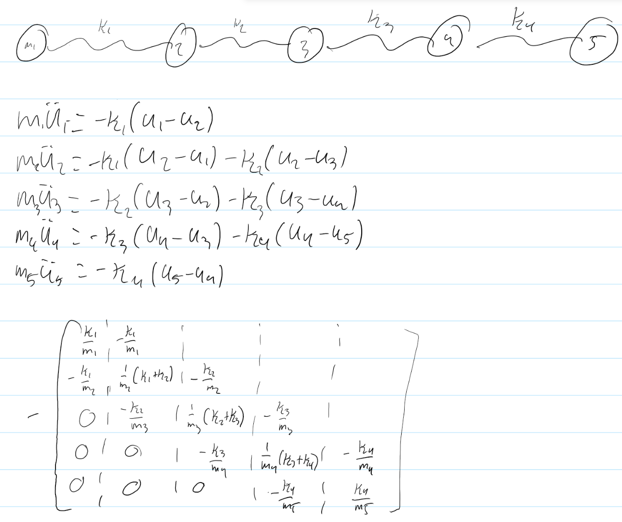
My code:

Code:

Note: Don’t pay to much attention to the validation, that is just to always convert the k and m to arrays so my code works for both scalars and arrays as inputs to k and or m.

class SpringChain1D():
    def __init__(self, n, k, m):

        if not (isinstance(n, int) or n <= 0):
            raise ValueError("n must be a positive integer")
        
        self.n = n

        # validate k
        if isinstance(k, (int, float)) and k > 0:
            self.k = np.full(n-1, k)  # Convert scalar k to an array
        elif isinstance(k, np.ndarray) and k.size == (n-1):
            self.k = k
        else:
            raise ValueError("k must be a positive scalar or an array of size n-1.")

        # Validate m
        if isinstance(m, (int, float)) and m > 0:
            self.m = np.full(n, m)  # Convert scalar m to an array
        elif isinstance(m, np.ndarray) and (m.size == n):
            self.m = m
        else:
            print(isinstance(m, np.ndarray), m.size, n)
            raise ValueError("m must be a positive scalar or an array of size n.")


        def construct_matrix(self):
            """
            Construct the tridiagonal matrix for the spring chain.
            The matrix is of size n x n, where n is the number of masses.
            The matrix is tridiagonal with the following structure:
                [ k[0]/m[0]   -k[0]/m[0]           0                  ...        0          ]
                [-k[0]/m[1]    (k[0]+k[1])/m[1]   -k[1]/m[1]          ...        0          ]
                [ 0           -k[1]/m[2]           (k[1]+k[2])/m[2]   ...        0          ]
                [ ...        ...                   ...                ...       -k[-1]/m[-2]]
                [ 0          0                     ...                -k/m[-1]   k/m[-1]    ]

            """
            self.matrix = np.zeros((self.n, self.n)) 
            np.fill_diagonal(self.matrix[1:], -self.k/self.m[1:]) # Fill lower sub-diagonal (previous mass)
            np.fill_diagonal(self.matrix[:,1:], -self.k/self.m[:-1]) # Fill upper sub-diagonal (next mass)

            # Fill main diagonal with the sum of the two adjacent springs devided by the mass
            diag = np.zeros(self.n)
            diag[:-1] = self.k
            diag[1:] += self.k
            diag /= self.m

            np.fill_diagonal(self.matrix, diag) # 

        construct_matrix(self)

    def eigenvalues(self):
        return np.linalg.eigvalsh(self.matrix)
    
    def plot_histogram(self, bins=40):
        fig, ax = plt.subplots()
        ax.hist(self.eigenvalues(), bins=bins)
        ax.set(title=f'Eigenvalue Histogram 1D spinchain N={self.n}', xlabel=r'$\omega^2$', ylabel='Frequency')
        return fig, ax

2. This is my histogram for the case where k&m are uniform.
   
   

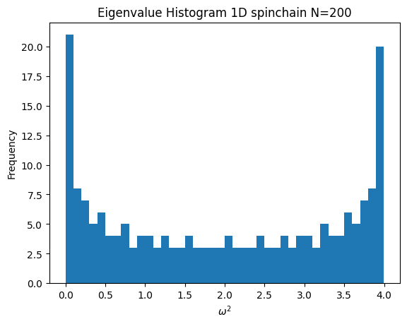
Code

N=200
chain = SpringChain1D(N, 1, 1)

chain.plot_histogram()

3. Where m_{2i} = 4 * m_{2i+1}
   
   

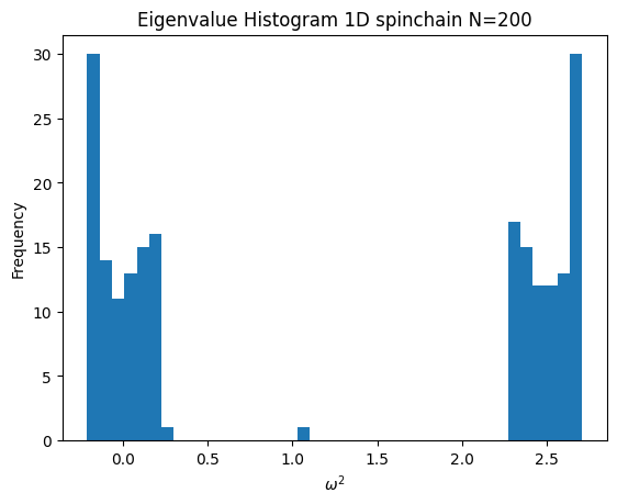
Code

m = np.tile([1,4], N)[:N]

chain = SpringChain1D(N, 1, m)
chain.plot_histogram()

4. Where k_{2i} = 2 * k_{2i+1}
   
   

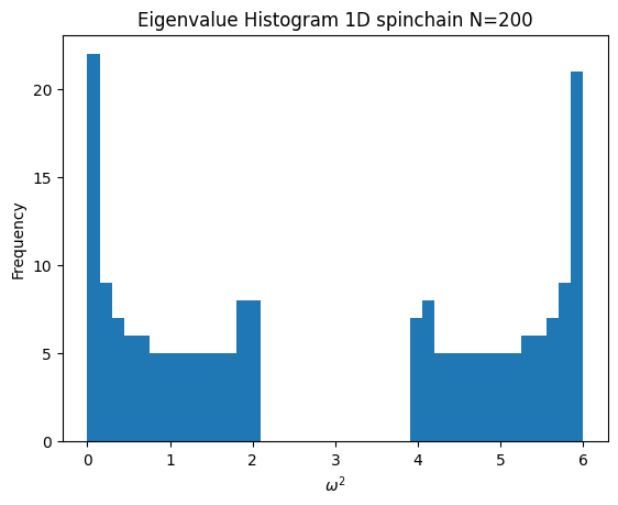
Code

k = np.tile([1,2], N-1)[:N-1]

chain = SpringChain1D(N, k, 1)
chain.plot_histogram()

[anton-akhmerov]

Nice code!

There is a subtle error though: the matrix you are diagonalizing isn’t Hermitian anymore (the upper offdiagonal terms are different from the lower offdiagonal ones). You can tell something is off because negative eigenvalues appear as well. There are two ways to fix the problem:

1. Use the generic diagonalization routine np.linalg.eig.
2. The more systematic approach is to solve a generalized eigenvalue problem, as I outline below.

Firstly, the equations we’re solving are of the form

M\omega^2 u = Ku,

where the M=M^T is the mass matrix, in our case a diagonal matrix with masses, and K=K^T is the stiffness matrix—a matrix with all the spring constants. So far we were converting this to a conventional eigenvalue problem by solving \omega^2 u = M^{-1}Ku. Once the masses aren’t constant, the matrix M^{-1}K isn’t symmetric anymore, though. An alternative option, however, is to use the generalized eigenvalue problem scipy.linalg.eigvalsh(K, M), which solves the eigenvalue equation above directly. It’s important to use scipy.linalg.eigvalsh because its numpy equivalent does not support generalized eigenvalues (numpy only has a minimal support of linear algebra).